In my last post, I gave you a theoretical knowledge of how Logistic Regression works. Along with the intuition, I provided you with a dataset to apply the theoretical knowledge on your own at first. In this post, I’ll explain you my approach to get a working model for the dataset I provided.
Let us first revist and have a deeper look into our dataset..because daahh..data is what matters the most for making predictions (Well, that’s a topic for another day).
Dataset Explained.
The provided dataset contains 4 columns, namely – ‘admit’, ‘rank’, ‘gpa’ and ‘gre’.
Where,
‘admit’ – represents whether a given student is provided with admit to the college(1) or not(0).
‘rank’ – represents the ranking of the college
‘gpa’ (or Grade Point Average) – represents the GPA of student in his previous academics.
‘gre’ (or Graduate Record Examination) – represents marks of student in the GRE exam.
Your task is to find a mapping from ‘rank’, ‘gre’ and ‘gpa’ to ‘admit’ so as to find whether a person will be admitted to the college or not.
If you haven’t yet read my last post, I recommend doing it before going ahead.
I strongly recommend to try to code it out yourself before looking at my solution.
Libraries used
We’ll be using Pandas for data extraction and NumPy for matrix operations. So, make sure you have a little knowledge of the stuff. Although, I’ll try my best to explain all the minor details.
So, grab your cup of coffee and follow along. It is going to be a little of a long ride.
Step 1 – Setting Up
We’ll be making a function called run, the main purpose of which will be to set up our data and call all the functions to perform gradient descent.
def run():
    #Collect data
    dataframe = pd.read_csv('binary.csv', sep = ',')
    data = dataframe.as_matrix()
    y = data[:, 0]
    X = data[:, 1:]
    #Scale Data
    X = feature_scaling(X)
    #Step 2 - define hyperparameters
    learning_rate = 3
    num_iters = 1000
    initial_theta = np.random.random(3)
    #train our model
    print('Starting gradient descent at theta = {0}, error = {1}, accuracy = {2}'
    .format(initial_theta, compute_error_for_separator_given_data(initial_theta, X, y), accuracy(initial_theta, X, y)))
    theta = gradient_descent_runner(X, y, initial_theta, learning_rate, num_iters)
    print('Ending gradient descent at Iteration = {0} theta = {1}, error = {2}, accuracy = {3}'
    .format(num_iters, theta, compute_error_for_separator_given_data(theta, X, y), accuracy(theta, X, y)))
In line 3, pd.read_csv() takes in two arguments for our purpose. First file name and second separator used in file (For those of you who don’t know, .csv means comma separated values). The function returns a dataframe. Converting this dataframe to a matrix (as in line 4) makes it easy to operate on data. In next two lines, we separate our labels (‘admit’) from features (‘rank’, ‘gpa’ and ‘gre’).
Rest of the functions will be covered one at a time.
Step 2 – Feature Scaling
From the heading itself its clear that we are targeting the black box we know nothing about at line 8 of run function.
While I’ll be discussing this topic in full depth in a future post, let’s look at what it means to scale the features here. Looking at the data, it is clear that ‘gre’ marks are in hundreds while both other features are in unit place. If this variation in feature is reduced, then we can reach to global optimum more easily and effectively. For this purpose, we will be using what we call Normalization. Doing this ensures that all the values are in the range of 0 and 1.
The formula we’ll be using here is:
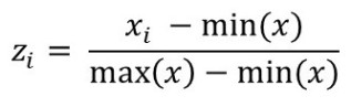
def feature_scaling(X):
    for i in range(X.shape[1]):
    X[:, i] = (X[:, i] - min(X[:, i])) / (max(X[:, i]) - min(X[:, i]))
    return X
This could have also been done using NumPy as
def feature_scaling(X):
    return (X - np.min(X, axis = 0)) / (np.max(X, axis = 0) - np.min(X, axis = 0))
Where the second keyword argument, as the name suggests apparently decides which axis to find the minimum or maximum on. Not using it will return minimum or maximum value out of the complete matrix.
Step 3 – Calculating Error
Before Calculating Error we need to define 2 more functions.
1. Sigmoid
2. Predict absolute value
Sigmoid
If you read my last post, then you definitely know what sigmoid function is and how we are going to use it here. So, without going into details lets jump to the code.
def sigmoid(z):
    return 1 / (1 + np.exp(-z))
Here, -z multiplies -1(to be precise, it just flips the sign bit) to each element of z. Then, np.exp(-z) applies element-wise exponential function on negative of z. The addition and division shown here works in element-wise manner.
Predict absolute value
Let us just directly jump to the code.
def predict_abs(theta, X):
    return sigmoid(np.dot(X, theta))
Here, np.dot(X, theta) performs simple matrix multiplication.
Now, since our base work is clear let us make our error computing function. As we already know, we use mean square error formula for this sake, i.e.,
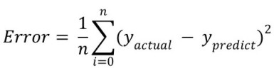
def compute_error_for_separator_given_data(theta, X, y):
    preds = predict_abs(theta, X)
    total_error = np.sum((y - preds) ** 2)
    return total_error / float(len(y))
We’ve scaled our features, we’ve computed the error.The only thing left to do is to run gradient descent on our data with our hyper-parameters.
Step 4 – Gradient Descent
From my last article we know that gradient descent works as:
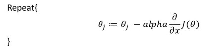
Ummm.. there is surely a call for separation of things to make the code easier to implement. So we will tackle each step of the Gradient Descent using a function called step_gradient.
def step_gradient(theta_current, X, y, learning_rate):
    preds = predict_abs(theta_current, X)
    theta_gradient = -(2 / len(y)) * np.dot(X.T, (y - preds))
    theta = theta_current - learning_rate * theta_gradient
    return theta
Going line by line, first we compute absolute predictions from given theta values and feature values. Then using them, we compute the partial differentiation of our cost function w.r.t theta and hence in the third line we find the value of new theta for current iteration of Gradient Descent.
Pretty Neat..!
So the only thing left is to iterate over this function a certain number of times as mentioned in our hyper-parameters.
def gradient_descent_runner(X, y, initial_theta, learning_rate, num_iters):
    theta = initial_theta
    for i in range(num_iters):
        theta = step_gradient(theta, X, y, learning_rate)
        return theta
Well, I don’t think this last piece of code needs any explanation though.
So, we are finally here..
We first setup our parameters and data.
Then we setup our probability calculating function – Sigmoid
After that, we hit the rock bottom of calculating the error
In the after math, we calculate new theta values from initial values using Gradient Descent.
Important Links:
Source Code: Github Link
Gradient Descent: Youtube Link
Part 1 of this Article: Logistic Regression – Let’s Classify Things..!!
PS: There might be many implementations far better than this. It will be great to see people raising issues in my repository on github. After all, we all are here to learn. And yeah this article was so delayed I’m sorry for I was really busy in some meetups and examinations. Many new articles coming this month.
Connect with me on:
![]()
![]()
![]()
