Linear Regression – Giving Best Fit Line

In my last post, I gave you an intuition of types of Machine Learning problems. Here, we’ll be undertaking the problem of regression(or real values fitting) which is a sub-category of Supervised Machine Learning.

But first things first!
We’ll be using Python for implementation along with its open source libraries like – NumPy, Pandas, Matplotlib and Scikit-learn. So, knowledge of basic python syntax is a must. At the end of the post, there is a list of all the resources to help you out.

So, here comes the time of a deep dive…!

What is Linear Regression?

Linear Regression is the problem of fitting the best possible line to the data. Woooaahh!!

Let us go through it step by step…

Why..?
Because we (Programmers) break down our work into smaller, simpler pieces
Step 1: Collect data
Step 2: Find a mapping from input data to labels, which gives minimum error… Magic of Mathematics!!
Step 3: Use this mapping to find label to new or unseen data-sets.

Wait! Don’t leave I know its MATHS, but we’ll make it easy.

How to find the Line of Best Fit?

A line that will fit the data in the best possible manner will be the line that has the minimum error. So, here is our objective – to minimize the error between the Actual Labels and Calculated Labels. And in order to accomplish it, we’ll be using one of the widely used algorithms in the world of ML – Gradient Descent.

So lets just dive right into the coding part:

Step 1: Collecting Data

For this example, we’ll be using NumPy to read data from an excel file – “data.csv”. The file contains data comparing the amount of hours a student studied and how much he or she scored.

def run():
 #Step 1 - Collect the data
 points = np.genfromtxt('data.csv', delimiter = ',')

Step 2: Finding The mapping

Our goal is to find a mapping between the hours studied and marks obtained, i.e.

y = mx + b

where,
x = amount of hours studied
y = marks obtained
m = slope of the line
b = y intercept

Well, this step has further sub-steps..

Step 2.1: Computing Error

To Compute Error at each iteration, we’ll be using the cost function(or objective function):

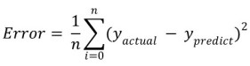
def compute_error_for_line_given_points(b, m, points):
 total_error = 0
 for ip in range(len(points)):
  x = points[ip, 0]
  y = points[ip, 1]
  total_error += (y - (m * x + b )) ** 2
 return total_error / float(len(points))

Looking at the mapping, it is clear that the only possible parts we can play around with to reduce the error are- m(the slope of the line) and b(the y intercept).

Step 2.2: Setting Hyper-parameters

In ML, we have certain parameters to tune in our model over the data we are analysing. These parameters are known as Hyper-parameters and they define certain terms that make sure our function(or model) fits data on a particular rate and in a particular way. We have a whole bunch of hyper-parameters with their own importance. More on this will be in a future post.

In our case, the Hyper-parameters that we must take into consideration are the Learning Rate, initial value of ‘b’, initial value of ‘m’ and number of iterations. Learning Rate defines how fast should our model converge. By converge, it means how fast model reaches the global optimum(in this case global minimum).

def run():
 #Step 1 - Collect the data
 points = np.genfromtxt('data.csv', delimiter = ',')

 #Step 2 - define hyperparameters
 learning_rate = 0.0001
 initial_b = 0
 initial_m = 0
 num_iterations = 1000

Well, then why isn’t Learning Rate big like a million?

The main reason being there must be a balance. If learning rate is too big, our error function might not converge(decrease), but if its too small, our error function might take too long to converge.

Step 2.3: Perform Gradient Descent

In this step, we will modify the value of y intercept ‘b’ and slope of line ‘m’ to decrease the value of the error (or objective function).

To do this, we will subtract the partial differentiation of our objective function with respect to b and m from former values of b and m respectively.

#Computes new values of b and m for a given iteration of gradient_descent_runner
def step_gradient(points, b_current, m_current, learning_rate):
 b_gradient = 0
 m_gradient = 0
 N = float(len(points))
 for i in range(len(points)):
  x = points[i, 0]
  y = points[i, 1]
  b_gradient += -(2/N) * (y - ((m_current * x) + b_current))
  m_gradient += -(2/N) * x * (y - ((m_current * x) + b_current))
 new_b = b_current - learning_rate * b_gradient
 new_m = m_current - learning_rate * m_gradient
 return [new_b, new_m]

#Finds the best fit line to the data.
def gradient_descent_runner(points, initial_b, initial_m, learning_rate, num_iterations):
 b = initial_b
 m = initial_m
 for i in range(num_iterations):
  b, m = step_gradient(points, b, m, learning_rate)
 return [b, m]

 

Step 3: Visualizing

Here, we will use Matplotlib – an open source library to plot graph of our mapping over the scatter plot of data.

def run():
 #Step 1 - Collect the data
 points = np.genfromtxt('data.csv', delimiter = ',')

 #Step 2 - define hyperparameters
 learning_rate = 0.0001
 initial_b = 0
 initial_m = 0
 num_iterations = 1000

 #Step 3 - train our model
 print('Starting gradient descent at b = {0}, m = {1}, error = {2}'
 .format(initial_b, initial_m, compute_error_for_line_given_points(initial_b, initial_m, points)))
 b, m = gradient_descent_runner(points, initial_b, initial_m, learning_rate, num_iterations)

 print('Ending gradient descent at Iteration = {0} b = {1}, m = {2}, error = {3}'
 .format(num_iterations, b, m, compute_error_for_line_given_points(b, m, points)))

 #Step 4 - Visualization
 x = [ix[0] for ix in points]
 y = [iy[1] for iy in points]
 y_predict = [m * ix + b for ix in x]

 plt.figure(0)
 plt.scatter(x, y)
 plt.plot(x, y_predict)
 plt.show()

 

Output : Graph Displaying the Best Fit line over the Data

To see a visual comparison between decrease in error and line fitting – go to link.

GitHub link to Source Code

Resources for further reading:

Python tutorial
NumPy tutorial
Matplotlib tutorial

PS: To get a good grip on the concept of Linear Regression visit this link.